
Gibbs Sampling: Python Implementation
Bayesian Networks are directed acyclic graphs used to model beliefs about the world. Abstractly, they represent the chance that a certain effect occurs given a set of possible causes, or the chance that a cause or causes led to an outcome. A Bayesian Network is comprised of variables connected through conditional dependence, which can be thought of as casual relationships. Each variable contains a domain of possible values and a joint probability distribution of the variable taking on specific values given the sets of values for its parents. From this model, one can infer the posterior probability that a set of query variables take on specific values, with or without a set of evidence (i.e. known values for specific variables).
Gibbs Sampling
When the Bayesian network is too complex (i.e., contains many variables and edges), exact inference methods such as Variable Elimination can become computationally inefficient. As an alternative, we will implement a Monte Carlo approach that combines two methods: Gibbs Sampling (GS) and Forward Sampling (FS).
Gibbs Sampling can be described as follows: Given the Markov Blanket of a random variable \(X\) (i.e., \(MB(X) = Pa(X) \cup Ch(X) \cup Pa(Chi(X))\)), \(X\) is independent of the remaining variables of the network and can be sampled independently. Therefore, Algorithm 1 describes the general GS process used to estimate the marginal probability distribution of each variable of the network based on the historic state of the network \(\textbf{x}\). In each iteration, we shuffle the order of variables an we sample a value for each non-evidence variable based on the probability distribution obtained by looking at the last observed values of it Markov Blanket. The \(\texttt{domain(X)}\) function retrieves a list of the possible values that the variable \(X\) can take. The \(\texttt{normalize(v)}\) function normalizes a probability distribution (i.e., a vector), such that the sum of its elements is 1.
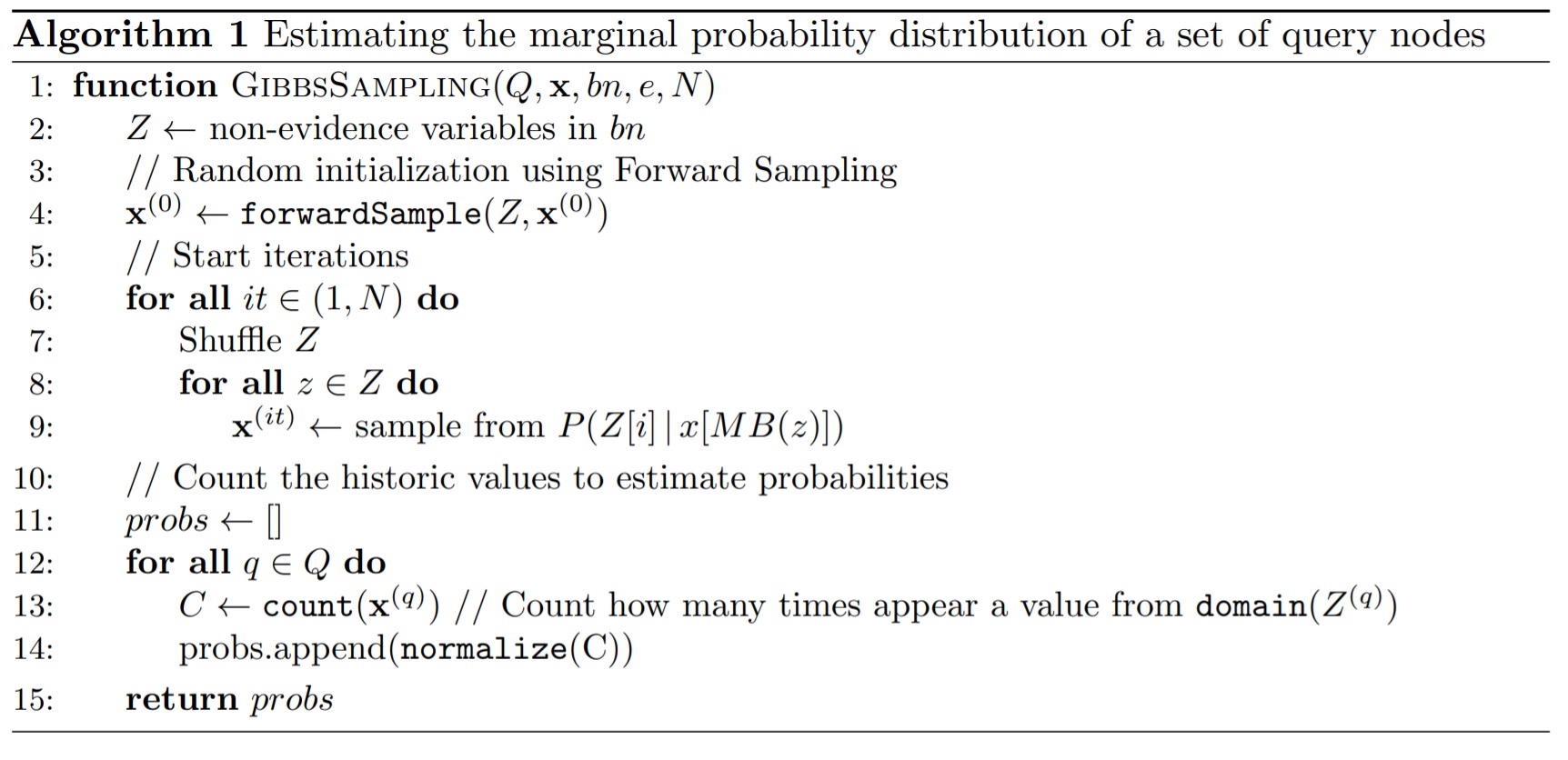 |
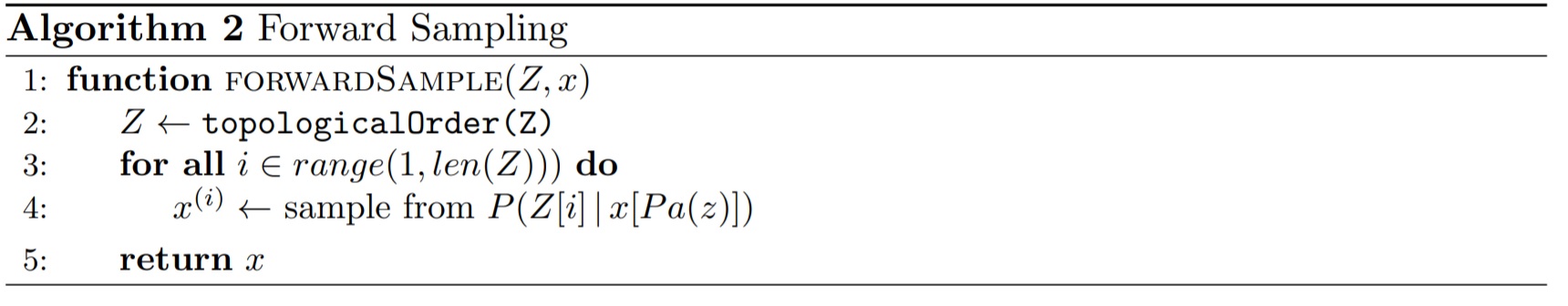
Note that Algorithm 1 calls the function \(\texttt{forwardSample}(z)\) (line 4) to obtain a sampled value for variable \(z\) using Forward Sampling. This method follows the previous definition that a variable \(X\) can be sampled based on the “given” (i.e., currently instantiated) variables of its Markov Blanket. Hence, FS first sorts the set of non-evidence variables in topological order using the \texttt{topologicalOrder()} function; that is, for every directed edge \(x \rightarrow y\) of the network, \(x\) has to appear before \(y\) in the ordering. Algorithm 2 shows the FS implementation. For every variable in the topological ordering, only its parents’ values have been instantiated, according to the previous state of the network $x$. Therefore, we sample a value for the \(i\)-th non-evidence variable from the probability distribution \(P(Z[i]\, | \, x[Pa(z)])\).
 |
Python Implementation
We create the \(\texttt{GibbsSampling}\) class that will be used to instantiate an object that will store some instance variables, such as \(\texttt{self.bn}\) and \(\texttt{self.query}\), and define the methods (both public and private) that will be used for the sampling process. We start with the initialization method and the main method of the class, \(\texttt{solve}\).
Note that the \(\texttt{solve}\) method takes two arguments: the graph used by our Bayesian Network (\(\texttt{bn}\)) and the set of query variables (\(\texttt{query}\)). For the sake of brevity, we are not providing the implementation code of the BN graph. However, \(\texttt{bn}\) is a graph that contains a set of interconnected nodes; each node is an object that represents a variable and has some important properties, such as \(\texttt{domain}\), which specifies the possible values the variable can take; \(\texttt{parents}\), the list of parent nodes; \(\texttt{children}\), the list of children nodes; and \(\texttt{probabilityDist}\), which is a matrix that specifies the conditional probability tables of each variable (see https://www.bnlearn.com/bnrepository/ for more information).
class GibbsSampling():
    """Class used to solve a query in a BN using Gibbs Sampling and Forward Sampling."""

    def __init__(self):
        self.K = 2000  # Number of iterations
        self.bn = None
        self.query = None
        self.nonev = []
        self.x = None

    def solve(self, bn, query):
        """
        @param bn: Bayesian Network model used for the inference process.
        @param query: Set of query nodes.
        """
        print('Starting Gibbs Sampling inference................................')
        # Initialize instance variables
        self.bn = bn
        self.query = query
        count = 0

        # Get list of non-evidence variables using Topological Order
        self.nonev = self.topologicalSort()

        # Initialize random values for each non-evidence variable
        self.x = np.empty((self.K, len(self.nonev)), dtype=object)  # Store the states of the network
        for i, nev in enumerate(self.nonev):
            self.x[0, i] = self.forwardSampling(nev)
            count += 1

        # Start iterations
        for it in range(1, self.K):
            # Shuffle non-evidence variables
            order = np.arange(len(self.nonev))
            random.shuffle(order)
            # Sample from each non-evidence
            for iv in order:
                self.x[it, iv] = self.sample_markov_blanket(self.nonev[iv], it)
                count += 1

        # Calculate the marginal probability distributions of the query nodes
        query_marginals = []
        for name in self.query:
            query_index = self.nonev.index(name)
            # Extract the sample history of the query node
            hist = list(self.x[:, query_index])
            # Count how many times each possible value appeared in hist
            counts = []
            for value in self.bn.nodeMap.get(name).domain:
                counts.append(hist.count(value))
            # Normalization
            counts = counts / np.sum(counts)
            query_marginals.append(counts)
            count += (len(counts) + 1)  # Add the number of sums and multiplications

        print('Gibbs Sampling process finished')
        print('Number of operations required = ' + str(count))
        return query_marginal
Note that within the \(\texttt{solve}\) function, the first step is to sort the variables of the graph in topological order. That is, we obtain a variable ordering such that every child appears after its parents. In order to do so, we use the function \(\texttt{topologicalSort}\) which uses a recursive helper function \(\texttt{topologicalSortHelper}\):
    def topologicalSort(self):
        """Method used to sort the non-evidence nodes in topological order"""
        # Mark all the vertices as not visited
        visited = [False] * len(self.bn.nodeMap)
        order = []

        # Perform recursion
        for n, i in enumerate(self.bn.nodeMap):
            if not visited[n]:
                self.topologicalSortHelper(i, visited, order)

        # Remove evidence nodes from the list
        for ev in self.bn.evidence:
            order.remove(ev[0])

        # Every node that has no parents will be first in the list
        for ev in order:
            if len(self.bn.nodeMap.get(ev).parents) == 0:
                order.remove(ev)
                order.insert(0, ev)

        return order

    def topologicalSortHelper(self, v, visited, order):
        """Recursive helper function used to obtain a topological order"""
        visited[list(self.bn.nodeMap).index(v)] = True  # Mark the current node as visited.

        # Perform recursion using children nodes
        adjacents = self.bn.nodeMap.get(v).children
        for i in adjacents:
            if not visited[list(self.bn.nodeMap).index(i)]:
                self.topologicalSortHelper(i, visited, order)

        # Push current node at the top
        order.insert(0, v)
Now, let’s implement the \(\texttt{forwardSampling}\) method, which is the Forward Sampling method defined in Algorithm 2 above that is used to sample the initial values of each non-evidence variable based on the values of its parents:
    def forwardSampling(self, nev):
        """Forward Sampling method
        @param nev: Name (string) of the query node.
        """

        ##############################################################################
        #  PART 1: Calculate the Conditional Probability of the node given its parents
        ##############################################################################

        # Get list of parents
        parents_current = self.bn.nodeMap.get(nev).parents

        prob_given_parents = []
        if len(parents_current) != 0:
            # Get values of the parents from previous iterations OR from evidence
            parents_values = []
            for par in parents_current:
                if self.bn.nodeMap.get(par).knownVal is not None:
                    parents_values.append(self.bn.nodeMap.get(par).knownVal)  # Add evidence value
                else:
                    # Find index of parents in the set of non-evidence variables
                    ind = self.nonev.index(par)
                    # Retrieve previous sampled value of this parent
                    parents_values.append(self.x[0, ind])

            # Calculate P(nev|parents(nev)) using the prob. dist. map of the current node
            for i in range(1, len(self.bn.nodeMap.get(nev).probabilityDist)):
                if self.bn.nodeMap.get(nev).probabilityDist[i][0] == parents_values:
                    prob_given_parents = self.bn.nodeMap.get(nev).probabilityDist[i][1:]  # Prob. dist.
                    break
        else:  # If the node has no parents, its conditional prob. is equal to the marginal prob.
            prob_given_parents = self.bn.nodeMap.get(nev).probabilityDist[1][1:]

        ##############################################################################
        #  PART 2: Sample according to the calculated probability distribution
        ##############################################################################
        sample = random.choices(self.bn.nodeMap.get(nev).domain, prob_given_parents)
        return sample[0]
Finally, let’s implement the \(\texttt{sample_markov_blanket}\) method used in Algorithm 1, which is used to sample the value of a non-evidence variable based on its Markov Blanket and the values observed in previous iterations of the algorithm, saved in \(\texttt{self.x}\). Note that the first part of the method is similar to the \(\texttt{forwardSampling}\) method; however, the probability distribution of a given variable given its parents is later affected by the observed value of its children and their parents in the second part of the algorithm.
    def sample_markov_blanket(self, nev, it):
        """Calculate P(nev | MB(nev))
        @param nev: Name (string) of the query node.
        @param it: Number of the current iteration (used to extract previous states).
        """

        ##############################################################################
        #  PART 1: Calculate the Conditional Probability of the node given its parents
        ##############################################################################

        # Get list of parents
        parents_current = self.bn.nodeMap.get(nev).parents

        prob_given_parents = []
        parents_values = []
        if len(parents_current) != 0:
            # Get values of the parents from previous iterations OR from evidence
            for par in parents_current:
                if self.bn.nodeMap.get(par).knownVal is not None:
                    parents_values.append(self.bn.nodeMap.get(par).knownVal)  # Add evidence value
                else:
                    # Find index of parents in the set of non-evidence variables
                    ind = self.nonev.index(par)
                    # Retrieve previous sampled value of this parent
                    if self.x[it, ind] is None:
                        parents_values.append(self.x[it - 1, ind])
                    else:
                        parents_values.append(self.x[it, ind])

            # Calculate P(nev|parents(nev)) using the prob. dist. map of the current node
            for i in range(1, len(self.bn.nodeMap.get(nev).probabilityDist)):
                if self.bn.nodeMap.get(nev).probabilityDist[i][0] == parents_values:
                    prob_given_parents = self.bn.nodeMap.get(nev).probabilityDist[i][1:]  # Probability distribution
                    break
        else:  # If the node has no parents, its conditional prob. is equal to the marginal prob.
            prob_given_parents = self.bn.nodeMap.get(nev).probabilityDist[1][1:]

        ################################################################################################
        #  PART 2: Calculate the Conditional Probability of the children of the node given their parents
        ################################################################################################

        # Get list of children
        children_current = self.bn.nodeMap.get(nev).children

        # For each children, calculate P(ch | Pa(ch))
        prob_given_markovblanket = np.array(prob_given_parents)
        for ch in children_current:
            # Get list of children parents
            ch_parents = self.bn.nodeMap.get(ch).parents
            # Get values of the parents from previous iterations OR from evidence
            ch_parents_values = [None] * len(ch_parents)
            curr_node_ind = 0
            for ip, par in enumerate(ch_parents):
                if par != nev:  # Assign parent value if the parent is not the node we're analyzing
                    if self.bn.nodeMap.get(par).knownVal is not None:
                        ch_parents_values[ip] = self.bn.nodeMap.get(par).knownVal  # Add evidence value
                    else:
                        # Find index of parents in the set of non-evidence variables
                        ind = self.nonev.index(par)
                        # Retrieve previous sampled value of this parent
                        ch_parents_values[ip] = self.x[it - 1, ind]
                else:
                    curr_node_ind = ip

            if self.bn.nodeMap.get(ch).knownVal is None:
                # Find index of current child in the set of non-evidence variables
                ch_ind = self.nonev.index(ch)
                # Retrieve previous sampled value of this child
                ch_value = self.x[it - 1, ch_ind]
            else:
                ch_value = self.bn.nodeMap.get(ch).knownVal
            # Retrieve index of this child in the domain list
            ch_column = self.bn.nodeMap.get(ch).domain.index(ch_value)

            # Calculate P(ch | Pa(ch)) using the prob. dist. map of the current child
            ch_prob_given_parents = []
            for dom in self.bn.nodeMap.get(nev).domain:
                ch_parents_values[curr_node_ind] = dom
                for i in range(1, len(self.bn.nodeMap.get(ch).probabilityDist)):
                    if self.bn.nodeMap.get(ch).probabilityDist[i][0] == ch_parents_values:
                        ch_prob_given_parents.append(self.bn.nodeMap.get(ch).probabilityDist[i][1 + ch_column])
                        break

            # Multiply previous and new prob. distribution
            prob_given_markovblanket = prob_given_markovblanket * np.array(ch_prob_given_parents)

        # Normalize dist.
        prob_given_markovblanket = prob_given_markovblanket / np.sum(prob_given_markovblanket)

        ##############################################################################
        #  PART 3: Sample according to the calculated probability distribution
        ##############################################################################
        sample = random.choices(self.bn.nodeMap.get(nev).domain, prob_given_markovblanket)

        return sample[0]
Thanks to Dalton Gomez for providing the Bayesian Networks definition at the beginning of this post.